 |
 |
|---|---|
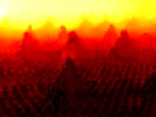
Semi-transparent images due to the presence of mist |
|
My name is Raanan Fattal and I joined the CS & Eng. department last year ('08). In this focus page I'll describe some of my recent work in Numerical Computing and its application to image processing. I'll start with describing two applications, haze removal and edge-preserving smoothing, followed by a short discussion about the numerical aspects behind the applications.
|
|
|---|---|
Semi-transparent images due to the presence of mist |
|
In many practical scenarios there is a layer of haze, mist, fog or dust that partially occludes the scene. In order to retrieve a clear view of the scene, showing it as if the medium is clear, we have to model the image formation process. Under certain simplification where we assume the light hitting the dust/fog particles and bouncing (scattering) to the viewer is uniform in space, the following equation can be used to explain the image,
I(x) = t(x)J(x) + (1-t(x)) A
This equation is quite simple: all it says is that a hazy image I(x), at each pixel x, is a sum of a haze-free image J(x), showing the light reflected from the surfaces in the scene, and the arlight A, which is the fog's whiteness that we assumed to be uniform in space. The scalar function t(x) is the transmission; a number between zero and one specifying the visibility fraction at every pixel x in the image. Unfortunately, we cannot recover J(x) given I(x) since we do not have enough constraints in the system; the images I(x) and J(x) considered here are 3D vectors representing the three color channels (red, green and blue) and therefore the input image I(x) provides us with only three equations per pixel whereas we have four unknowns, three in J(x) and one in t(x). This is the case at every pixel x and it adds up to a huge amount of uncertainty, millions of undetermined degrees of freedom in a single image. This means that we have to derive a more restricted model; a model that involves less degrees of freedom yet is still able to express the input image. In my work, I further assume that pixels in the image locally share the same intrinsic color, their reflection coefficients (albedo). This assumption reduces the number of unknowns to 2n+1, but at the same time reduces the number of equations to 2n, where n is the number of pixels that share the same reflectance values. This significant reduction in the ambiguity is still not enough; we need one more constraint in order to fully pose the system. The remaining one-dimensional uncertainty, that we have at each pixel, has a very simple interpretation: we cannot say how much of the airlight color is present in the surface color (reflectance coefficients), i.e., we can't tell whether a given surface color is saturated yet occluded by a dense layer of fog or it has a faint color (similar to the airlight color) seen through an almost clear medium. Hopefully, by now the reader is interested enough as to read the full report on the problem. Here are some results obtained once this final uncertainty is resolved:
|
|
|---|---|
 |
 |
 |
 |
Top to bottom are the: input I(x), output J(x), and the transmission t(x) |
|
The second aspect of this work, aside of deriving a mathematical model, is solving the resulting equations. In many cases, the equations we get from practical problems cannot be solved analytically and require the aid of a computer in order to compute an approximate solution. This challenging and fascinating field is called numerical or scientific computing and I'll try to give you some flavor of it. A well-known equation, the inhomogeneous Laplace equation, is used in the dehazing problem (in a regularization step, not mentioned above) and in many other applications such as edge-preserving image smoothing and sparse-data interpolation. This equation results from minimizing the derivatives of a function I(x) in a spatially-dependent manner, i.e., minimizing the following functional,
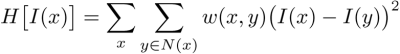
where I(x) is now a single-color image (e.g., a gray-scale image) and N(x) is the set of the pixel x's neighboring pixels. The function w weighs each pixel difference differently in space. The image I(x) obtained from this minimization "tries" to remain unchanged at points where w is high. Note that the trivial solution of I(x)=0 everywhere is avoided by fixing a few values of I(x) to be non-zero. For example, in another work (with collaborators: Zeev Farbman, Dani Lischinski and Richard Szeliski), we define w based on some input image T(x) such that w high when T(x) is flat and low where T(x) changes considerably. The solution I(x) from this minimization is piecewise smooth and shares the same edges as the input T(x). This operation is important for many applications such as detail enhancement, dynamic-range compression and image simplification (see here the paper). Solving this minimization boils down to solving a large system of linear equations (one variable per pixel) which is not easy when the weighting function w shows a large ratio between its highest and lowest values. In terms of numerical linear algebra one would say that the matrix describing this linear system is poorly-conditioned. Effectively, this means that generic iterative linear solvers, such as Gauss-Seidel and Conjugate Gradients, will not be efficient and require many iterations to converge to a solution.
 |
An image and a detail-enhanced ouput produced via an edge preserving smoothing. The detail enhancement is achieved by adding the difference between the input image and the smoothed image to the input image. |
|---|
The reason for this "stiffness" can be explained in terms of eigenvectors and eigenvalues (you can refresh these terms here). The point is that large ratios in w translate into a large ratios between the highest and lowest eigenvalues of the minimizing matrix. This amplifies certain components in the error, during solution, and weakens the rest. As such, iterative solvers do not "sense" these weak components and compute the solution only over a limited subspace--the one spanned by the eigenvectors that correspond to the large eigenvalues. Since we already gathered some intuition about the objective functional itself, we can get an idea as to who are the amplified and attenuated error components. The functional H penalizes functions with large pixel differences and smooth functions receive low scores. One can easily show that these scores are an outcome of the function's composition in terms of the eigenvectors and reach the following conclusion: the rapidly-changing functions correspond to the amplified error components that get quickly solved while the smooth functions correspond to the error components that get attenuated and are therefore solved slowly. This implies that after a few iterations of Gauss-Seidel (a particular iterative solver) we expect the solution to be differing from the true solution by a smooth function.

In order to cope with this problem one has to separate the different component based on their smoothness and solve them separately, which will achieve a constant rate of convergence at all the error-components. This is precisely what the Multi-Grid method does; effectively it generates new basis functions at different scales (and hence at different levels of smoothness) and solves the equation at each linear subspace separately. The Multi-Grid method is known to be one of the fastest (if not the fastest) methods for solving this type of linear equations. However, the construction of these basis functions is still a matter of scientific investigation since the convergence rate depends on how extreme the weighting function w changes as well as on other singularities it may show (such as nearly-isolated sets of strongly coupled variables). There are several strategies for constructing a good basis (and doing so efficiently). The direction I am considering is to compute the basis functions by solving local optimization problems that resemble the global problem as much as possible. This type of equations are also used for modeling different physical phenomena as well as for computing the maximum likelihood estimators of Gaussian Markov field models.
 |
 |
|---|---|
Graphs showing a few basis functions computed at a coarse level (i.e., smooth components). These functions adapt to an extreme connectivity scenario; there's a vertical line weighted by w=1/10000 separating two strongly connected domains (with w=1). |
|